IoT Devices Lab Series 5 - Getting Started with Sensors and Micropython on the ESP32

Introduction

In this lab, you'll be working with two types of sensors (analog and digital) connected to your board. You'll learn how to manage the ESP32 ADC as well as understand and practice with the I2C protocol.

Pre-requisites

The tutorial assumes you have Python3 installed in your machine, and that you have access to the following materials:

• A development environment with direct USB access (your laptop)
• An ESP32-based development board
• A Capacitive Moisture Sensor 1.2 (analog capacitive sensor)
• A Grove Temperature Sensor (NTC-based analog sensor)
• A glass of water
• A multimeter
• Jumper wires
• A USB-A to micro USB cable to connect the dev board to your computer.
• Sensirion SHT30 Datasheet

Analog sensors

Using a capacitive moisture sensor

The capacitive moisture sensor used in the lab has a NE555 93M timer (datasheet) that operates at 5V. This is related to the the sensor not having a voltage regulator, which means it needs a timer that works with 5V as input. This means that the output voltage will go north the max 3.3V handled by ESP32 GPIO inputs, which means we'll need to lower it down. What's more, the ADC in the ESP32 accepts voltages up to 950mV without attenuation, meaning that we'll need to actually make sure our voltage does not exceed that number.

Measuring the range of the output voltage of the sensor when dry, it goes as high as 4.7V. The most common technique to adjust the output voltage of the sensor is using a voltage divider. Instead of using a pair of resistors with given values that lower down the voltage to what we want, we'll use a more convenient device, a potentiometer.

We're picking up here a 105 potentiometer (up to 1M total resistance) because the sensor is expecting to find a high output impedance, as the current that is capable to source is very small. If we were to use lower resistance values will cause more current to be consumed, and that's bad because the sensor won't be able to source that much.

As we said, the potentiometer is being used as a voltage divider. Of course, we're not dealing with an unloaded voltage divider but rather a loaded one, so what's why it's so important to pay attention to the currents involved.

Let's try this out to understand how to use our sensor.

Understanding the sensor output

Making the connections

• Connect the 5V pin of the ESP32 to the Vin of the Capacitive Soil Sensor (CCS)
• Conect the GND rail of the breadboard to the GND pin of the CCS
• Connect the Aout of the CSS to a jumper wire, and leave it unconnected.

Get a glass of water. Connect a multimeter between GND and the unconnected jumper wire. Put the multimeter reading to Vcc observe what the voltage ranges are when the sensor is dry and when you submerge the sensor in different degrees into the glass of water.

Adjusting the voltage divider

Making the connections

• Connect the 5V pin of the ESP32 to the Vin of the Capacitive Soil Sensor (CCS)
• Conect the GND rail of the breadboard to the GND pin of the CCS
• Connect the Aout of the CSS to the pin one of a potentiometer (a 105, for example)
• Connect the pin 3 of the potentiometer to GND
• Connect the pin 2 of the potentiomenter to a jumper wire, and leave it unconnected.

Connect a multimeter between GND and the pin 2 of the potentiometer. Put the multimeter reading to Vcc and adjust the potentiometer until you're below 950mV. Then, disconnect the multimeter from GND and pin 2 of the potentiometer and connect it to the pin 32 of the ESP32.

Writing our code

The capacitive sensor will output the biggest voltage when it's dry. Because we've adjusted our signal to be less than 950mV, that means we won't need any attenuation in the ADC (see possible attenuation values), so the following code will give us humidity lectures:

from machine import Pin, ADC
from time import sleep_ms

sensor0 = ADC(Pin(32))
# No attenuation is the default, and in any case would be equivalent to:
# sensor0.atten(ADC.ATTN_0DB) 

for i in range(120):
    print(sensor0.read())
    sleep_ms(500)

Calibrating the sensor

Get the glass of water and test the sensor out. When dry, the ADC should output a max of 4053, and when fully submerged in water, down to 1660. With these numbers in mind, we can now adjust our small program to give us a percentage of humidity to return:

from machine import Pin, ADC
from time import sleep_ms

sensor0 = ADC(Pin(32))
# No attenuation is the default, and in any case would be equivalent to:
# sensor0.atten(ADC.ATTN_0DB)

# Modify these values based on previous tests
dry = 4053
wet = 1660

def humidity(x):
    # This is the inverse of dryness, as dry is the biggest value
    humid_value = 100 - 100*(x - wet)/(dry - wet)
    return humid_value

for i in range(120):
    print("{}% humidity", humidity(sensor0.read()))
    sleep_ms(500)

Using an analog temperature sensor

Let's practice now with another analog sensor, in this case a Negative Temperature Coefficient Thermistor embedded in a small PCB. Our sensor is the Grove Temperature Sensor 1.2, taken from a SeeedStudio IoT kit.

A short look at the sensor feature will tell us this sensor is fed by 3.3V, an returns a range of voltages that is in relation to the temperature the NTC Thermistor is sensing.

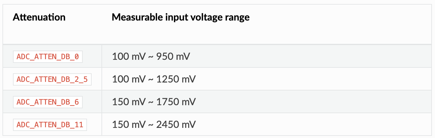
Now, we know that the ADC in the ESP32 expects an input range in the [100mv, 950mV] interval with no attenuation. When there's attenuation configured, the range changes following this table:

Now, the behavior of the ADC in the ESP32 is more or less linear depending on the attenuation and range we're in. In the following graph, we can see that the ADC behaves perfectly linearly in the 0dB attenuation setting, but in the 11dB setting, that would give us more margin to play with when it comes to sensor outputs that are fed by 3.3V, we see non-linearity at the end of the graph.

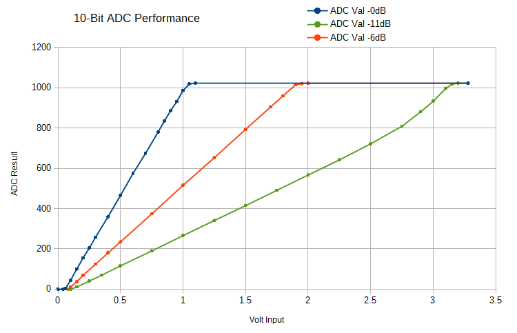
Actually, with 0dB attenuation the non linear behavior starts around 2450mV, and that's why the ADC spec mentions that upper limit. That doesn't mean though that our input cannot take more than that. It probably means that the measurement we're getting from the output of the ADC is not precise.

There's an additional function read_uv() exposed in MicroPython that returns a calibrated input voltage in milivolts, valid in the linear range of the ADC. Unfortunately, the method was added quite recently to MicroPython and didn't make it for MicroPython version 1.18. As of the writing of this document, this is the firmware version that we're using.

With all this in mind, let's try the sensor first:

Understanding the voltage output

Making the connections

• Connect the 3.3V pin of the ESP32 (or positive power rail) to the Vin of the sensor
• Conect the GND rail of the breadboard to the GND pin of the sensor
• Connect the Aout of the sensor to the pin one of a potentiometer (a 105, for example)
• Connect the pin 3 of the potentiometer to GND
• Connect the pin 2 of the potentiomenter to a jumper wire, and leave it unconnected.

Now, adjust the potentiometer until the voltage output is more or less in the range of the 11dB attenuation range. Leave the potentiometer at that position and proceed to make the connections with the ESP32.

Connecting the sensor to the board

Making the connections

For this, well use the previous potentiometer adjusted for the voltage range that we determined previously.

• Connect the 3.3V pin of the ESP32 (or positive power rail) to the Vin of the sensor
• Conect the GND rail of the breadboard to the GND pin of the sensor
• Connect the Aout of the sensor to the pin one of a potentiometer (a 105, for example)
• Connect the pin 3 of the potentiometer to GND
• Connect the pin 2 of the potentiomenter the an ADC-enabled pin in the ESP32.

As for the code, just for the sake of demonstration of the Steinhart-Hart NTC equation, we'll provide the following code considering our sensor is providing 3.3V output and that we don't care about non linearities in the ADC as we'll be unlikely hitting the max temperatures that the sensor can give us:

from machine import Pin, ADC
import time, math

raw = ADC(Pin(32))
raw.atten(ADC.ATTN_11DB) # Max attenuation to process up to 3.3V input
B = 4275 # B value of the thermistor
R0 = 100000 # R0 = 100k

def temp(reading):
    # ESP32 ADC specific, resolution is 12bit
    R = 4096.0 / reading - 1.0
    R = R0*R
    # Temperature is in Kelvin, converting
    temperature = 1.0/(math.log(R/R0)/B + 1/298.15) - 273.15
    return temperature

while True:
    print("Temperature: ", temp(raw.read()), "C")

SHT3x

The STH3x is a low cost version of the quite popular Sensirion series SHT30. It is a high quality combined humidity and temperature sensor that is manufactured in several versions. Our version is the one using the I2C protocol, which makes it a digital sensor, something more interesting as it will provide more interaction with our code.

For this lab, we'll be heavily relying on two sources: - The official Sensirion Datasheet SHT3x-DIS Datasheet - MicroPython's I2C Class documentation

The datasheet includes all the information about the sensor that we'll need to use it: feature, I2C addresses and commands, physical formulas, and other operating parameters of the sensor. The MicroPython documentation will give us a hint of the I2C features that we have available in the firmware deployed on our ESP32.

SHT3x board

For this lab, we've considered a couple of boards mounting this sensor:

• SHT3x generic board
• DFRobot's SHT3x board

The first is quite cheap, but fully functional The second is more expensive, but it's a slightly better designed board with good documentation. For the following examples we'll move on with the first one, a board that exposes the following pins:

• Vcc: 3.3 Volts
• GND: Ground
• SCL: I2C's clock channel
• SDA: I2C's data channel
• AL: Alarm pin
• AD: Addres change pin

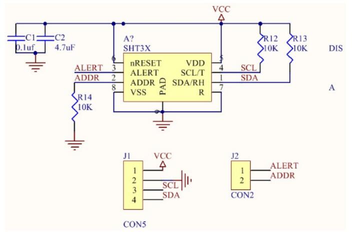
The schematics of the sensor are the following:

SHT3x Schematics

ESP32 I2C Pinout and physical connections

As mentioned before in other labs of this Series, we'll be using an Espressif ESP32 DevKitC-1 board, based on the ESP32 32D chip. For this board, the pinout we'll be using for I2C communication is:

ESP32 WROOM 32D Pinout

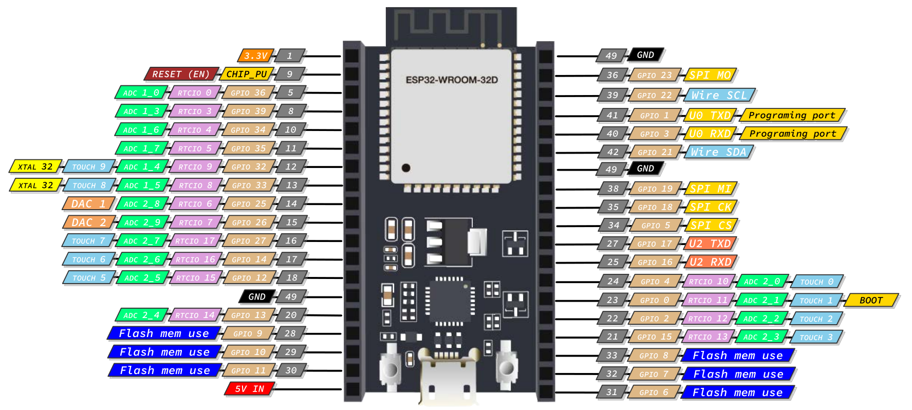
As you can see in light blue, the relevant I2C GPIOs that we'll need to connect to our sensor board are:

Vcc	GND	SDA	SCL
3.3v	GND	21	22

For the purposes of what we're trying to accomplish here, any other ESP32 device will do, although the pinout may be different. Keep that in mind when following through the next sections of this lab. Leave the AL and AD pins unconnected as you won't be using them in this lab.

Addressing the sensor

Once the sensor board is connected to the ESP32, connect your computer and the ESP32 with a USB data cable, and get a MicroPython REPL (if not, recheck the steps where you flashed the device's firmware and try again). The following will be a series of code lines that you're expected to enter in MicroPython's REPL.

As mentioned before, Micropython's I2C library documentation can help us along the way, so feel free to navigate the different constructors and methods that we'll be using during this lab.

First, import necessary libraries:

from machine import Pin, I2C

Once the I2C module is imported, let's use the I2C class constructor to set up a connection to the I2C bus:

i2c = I2C(1, freq=400_000, scl=Pin(22), sda=Pin(21))

We're using here the id value 1, as it works well for the ESP32, establishing the maximum working frequency for I2C in fast mode (400kHz), and setting up the pins we'll be using for I2C communication. We're using this specific frequency as we can check in the datasheet (section 3.2) that the sensor is expecting I2C fast mode to be used. The ESP32 chip we're using supports up to 1MHz, but because we're not sure about the quality control of pull up resistors and capacitance along the lines, we'll stay safe and use 400 kHz.

Next, let's scan the bus for slave devices:

addr = i2c.scan()
print(addr)

This should output:

[68]

The return list contains the decimal numbers representing the address identifiers of the slave devices connected to the bus. The list should contain only one element as we just connected one sensor to the MCU:

addr = addr[0]
hex(addr)

This should output:

0x44

This address is well known, as it is the default address used by the SHT3x chip as documented in the datasheet (section 3.4, table 8). If the pin AD is soldered in your sensor board, and you're connecting that pin to Vcc, then the address to use would be 0x45.

Requesting the sensor to take a measurement (writing to the sensor)

To know what's next, let's continue reading the datasheet. Moving to section 4 in the document, we can see in subsection 4.3 that we cand select a mode where we can issue measure commands to the sensor either in one shot or in streams of measurements.

We'll focus in the one shot acquisition mode. In this mode one issued measurement command triggers the acquisition of one data pair, each data pair consisting of one 2 bytes temperature reading and another 2 bytes humidity value, in this order. During transmission of these values, as per the datasheet, we should expect each data value to be followed by a CRC checksum.

Table 9 has the detail of the measurement commands in this specific mode. The command we'll need to use next is highlighted in red:

Measurement request

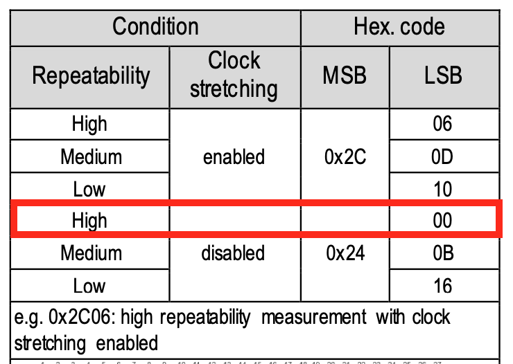
A longer measurement in the sensor will typically mean a better one, though the energy consumption of the sensor will go up. As we're prototyping and using our sensor connected to USB to a power supply, and because our focus is on learning the internals of the I2C protocol, we'll focus on precision and select a high repeatability.

The other option that appears in the table is clock stretching. Altough clock stretching is an interesting technique that may allow us not to run into timout problems, we'll keep it simple and let the master control the clock at all moments.

So, the next command to issue is to tell our sensor to take a measurement. This implies sending the two bytes outlined before:

status = i2c.writeto(addr,b'\x24\x00')
print(status)

This should output the number of bytes written:

2

Reading sensor data

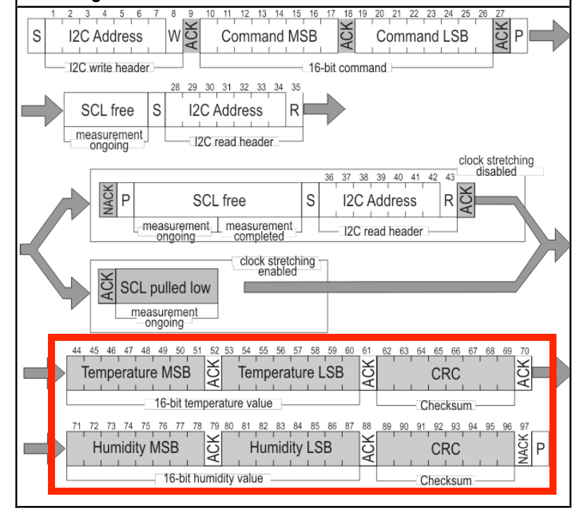
Next, we need to read the sensor values we've gotten back from Again, according to Table 9 in the SHT3x datasheet, we should expect 2 bytes of data per type of sensor (Temperature, Humidity), and one CRC checksum per type of measurement. That amounts to a total of 6 bytes, as we can see in the figure:

One Shot Measurement

Given all this information, we'll do the request for reading and the actual capture of sensor data from the I2C bus with just one command:

1. Address the slave device and pass a Read command in that first byte (this is what readfrom(addr will do)
2. Listen for a response sequence, that according to the SHT3x datasheet, should be 6 bytes long (and that's the 6 in readfrom(addr, 6) is coming from).

response_databytes = i2c.readfrom(addr, 6)

From the last figure, we know we're obtaining the MSB and LSB for the Temperature, then a CRC, and then the MSB and LSB for the Humidity, followed by the corresponding CRC.

We first join both MSB and LSB from the two measurements, by performing a shift on the MSB and then adding the LSB doing a bitwise OR:

temperature_raw = response_databytes[0] << 8 | response_databytes[1]
humidity_raw = response_databytes[3] << 8  | response_databytes[4]
print(temperature_raw, humidity_raw)

These are going to be raw measurements expressed in decimal.

Translating sensor data to Temperature and Humidity values

Our final step is to get sensor data in the proper units. Temperature and humidity conversion formulas given the binary measurements obtained from the sensor come from section 4.13 of the SHT3x Datasheet:

\[ T=-45+175\cdot\frac{S_T}{2^{16}-1} \]

\[RH=100\cdot\frac{S_{RH}}{2^{16}-1}\]

where \(S_{RH}\) and \(S_T\) denote the raw sensor output for humidity and temperature in decimal obtained from the sensor. With this, we can finally obtain the physical quantities from the sensor:

temperature = (175.0 * float(temperature_raw) / 65535.0) - 45
humidity = (100.0 * float(humidity_raw) / 65535.0)
sensor_data = [temperature, humidity]
print(sensor_data)

What is printed should be in a reasonable range given the temperature and humidity conditions of your city in the season you're performing the experiment.

Observing the signal with a Logic Analyzer

Additional links

• Understanding RC circuits
• MicroPython Moisture Sensor Calibration Library
• Non linearities in ESP32 ADC input
• NTC Thermistor Datasheet
• ESP32 Forum discussion on ADC linearity and corretions
• ESP32 Forum: what are the ACD input ranges?
• Understanding the effect of pull up resistors in I2C frequency limits